
One of the most crucial roles in business finance is the daily management of the company's books, which involves making sure that costs and revenues are recorded, accounts are reconciled, and data is inputted accurately. Accounting is a crucial task in managing your company's finances since it keeps you informed and ready to handle financial obligations. While some companies would rather use accounting software or employ a certified public accountant, a small company or startup may decide to build a bookkeeping system using Microsoft Excel.
Having the right tools is crucial when it comes to accounting in order to guarantee accuracy and effectiveness. Excel has established itself as a crucial accounting tool. Excel's extensive functionality enables accountants to perform all necessary calculations, from the simplest to the most complex, with just a few clicks and selections. Microsoft is always developing new functions for Excel that are not only crucial but also make accounting simpler and more accurate. In this post, we discuss the best accounting-related Excel functions.


Excel Formula List for Accounting
Excel is a powerful tool that accountants can use to automate repetitive computations, and store and manage financial data. Gaining or honing your accounting skills can be facilitated by learning practical Excel formulas. In Microsoft Excel, you may solve computations using both formulas and functions. Formulas are calculations that the user defines. Excel's formula might read =B2+B3+B4 if a user wanted to combine the numbers in cells B2, B3, and B4. In Excel, functions are pre-built formulas. The functions SUM and AVERAGE are two examples.
Asset Depreciation
Asset depreciation can be calculated by accountants to determine how much value an asset loses over time. Excel provides five ways to determine asset depreciation:
-
DB(cost, salvage, life, period, month): The decline balance depreciation method can be used to reduce an asset's value by a fixed percentage. The month value is optional.
-
SLN(cost, salvage, life): The straight-line depreciation calculation can be used to demonstrate an asset's value lowering by a fixed period of time over its life.
-
DDB(cost, salvage, life, period, factor): Double decline balance depreciation is another Excel method that can double the rate of straight-line depreciation. The factor value is optional.
-
VDB(cost, salvage, life, start period, end period, factor, no switch): Variable decline balance can show depreciation over a user-specified period. The factor and no switch values are optional.
-
SYD(cost, salvage, life, per): The sum-of-years' digits depreciation can also show the declining value of an item.
Learn more about accounting with accountancy tuition near me on Superprof.
Annual Interest Rate
You can use the RATE function in Excel to calculate the annual interest rate on a loan. Formula: RATE(nper, pmt, pv, fv, type, guess)
-
Nper: This is the number of payment periods.
-
Pmt: This stands for the amount paid toward a loan each year.
-
Pv: This represents the loan's present value.
-
Fv: You can optionally include the loan's balance after the final instalment.
-
Type: This optional argument stands for when a loan payment is due. A one can be used for the beginning of the pay period and a zero can be used for the end.
-
Guess: This optional value stands for the Excel user's guess for the rate. This value defaults to 10%.
Compound Interest
Compound interest is the inclusion of interest in a loan's principal sum. Accountants use a compound interest formula in Excel to find an investment's future value. Formula: p * (1+r)^n
-
P: This stands for the principal loan amount
-
R: This is the loan's interest rate.
-
N: This is the investment period for the loan.
Mortgage Payments
Accountants use the PMT function to determine the cost of a mortgage payment. Formula: PMT(rate, nper, pv, fv, type)
-
Rate: This is the interest rate for the loan.
-
Nper: Nper stands for the number of loan payments due.
-
PV: This is the loan's principal amount.
-
FV: This value represents the cash balance after the last instalment. This value is optional. If you don't include an fv value, it defaults to zero.
-
Type: This represents when the loan payment is due. This value is also optional. A value of one represents the beginning of the payment period and a value of zero represents the end of the payment period.
Future Value of Investments
Accountants can use the future value function to find the value of an investment in the future. Formula: FV(rate, nper, pmt, pv, type)
-
Rate: This represents the interest rate per period.
-
Nper: Nper is the number of payment periods.
-
Pmt: This is the value of the payment made each period.
-
Pv: This optional value is the value of future payments at present.
-
Type: This optional parameter shows when a payment is due. You can use zero for the end of a payment period and one for the beginning.

Effective Annual Interest Rate
Accountants can use the EFFECT formula to determine the effective annual interest rate on a loan. Formula: EFFECT(nominal_rate, npery)
-
Nominal_rate: This is the nominal interest rate or the interest rate before inflation.
-
Npery: This is the number of annual compounding periods or the number of times per payment period that interest is added to a loan.
Discover accountancy tuition near me when you search on Superprof.
Fixed Loan Payment Interest
You can calculate the portion of interest on a loan payment that's fixed using the IPMT function in Excel. Formula: IPMT(rate, per, nper, pv, fv, type)
-
Rate: This is the interest rate for the loan.
-
Per: This is the period for the interest.
-
Nper: Nper stands for the number of loan payments due.
-
PV: This is the loan's principal amount.
-
FV: This value represents the cash balance after the last instalment. This value is optional.
-
Type: This represents when the loan payment is due. This value is also optional.
Cash Flows
You can use the MIRR function in Excel to calculate cash flows for a company. It stands for modified internal rate of return. Function: MIRR(cash_flows, finance_rate, reinvest_rate)
-
Cash_flows: The first parameter refers to cells that contain cash flows.
-
Finance_rate: This is the rate of return (or the discount rate), shown as a percentage.
-
Reinvest_rate: This is a percentage that represents the interest rate received on reinvested cash flows.
Internal Rate of Return
Accountants can use the IRR function to calculate the internal rate of return for cash flows. Function: IRR(values, guess)
-
Cash_flows: This is a reference to cells that contain a company's cash flows. For example, (D6:D11).
-
Guess: This optional parameter is the user's guess for the internal rate of return.
Accrued Interest
Accountants can use the ACCRINT function to calculate the accrued interest over a time period for security, like a bond. Function: ACCRINT(id, fd, sd, rate, par, freq, basis, calc)
-
id: This is the issue date for the security.
-
fd: This represents the first interest date of the security.
-
sd: This is the settlement date for the security.
-
rate: This represents the security's interest rate.
-
par: This is the security's par value or its face value.
-
freq: This is the number of payments per year.
-
basis: This optional parameter controls how Excel counts days using this function.
-
calc: This optional parameter controls how Excel calculates the method.
Discover more tips and tricks to improve your accounting skills with an accounting class on Superprof!
Top Accounting Functions in MS Excel
AGGREGATE
The AGGREGATE function allows you to sum (along with other functions like AVERAGE, COUNT, MAX, MIN, etc.) a range of cells while ignoring any cells that may contain errors as well as ignoring hidden values due to hiding rows and/or columns. AGGREGATE is 19 separate functions packaged into a single function with additional features thrown in for good measure. When you write a formula using the AGGREGATE function, you use a code number to indicate which of the 19 functions you wish to use.
Selecting the appropriate option value will alter the way AGGREGATE behaves when encountering errors, hidden rows, or even other AGGREGATE functions. This is a great way for accountants to create subtotals and grand totals whereby the grand totals ignore the subtotals, avoiding the issue of double counting. These options are also useful when you are filtering tables and you don’t want the hidden rows to be included in the aggregations. The SUM function (along with other functions like AVERAGE, COUNT, MAX, MIN, etc.) would continue to include the values in the filtered/hidden rows.
ROUND
The ROUND function allows you to round your results to a set number of decimal places. When we perform calculations, often the result is displayed to a level of precision beyond our needs. To ensure that a result is only ever displayed to a set level of decimal precision, we can enclose the calculation in a ROUND function and define the number of decimal places, such as 2 decimal places or rounded to a whole number. A lesser-known ability of the ROUND function is that you can round UP in a “left of the decimal” fashion. This is useful when you are representing very large numbers, but you only need precision to a certain level.
EOMONTH
The EOMONTH (End of Month) function accepts a date or a reference to a cell holding a date and produces a new date that is the last day of the month for a set number of months forward or backwards in time.
EDATE
The EDATE function allows you to move a set number of months forward or backwards in time based on a specified date. If you need to calculate the N-number of months in the past, define the “Months” argument as a negative value.
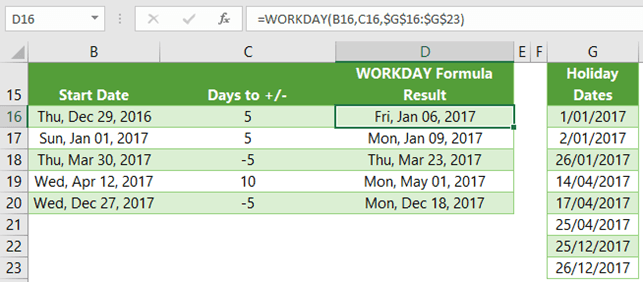
WORKDAY
The WORKDAY function is ideal for calculating a set number of days forward (or backward) in time but skipping the weekends and possibly holidays. There are two versions of the WORKDAY function:
- WORKDAY: An older version that defines Saturday and Sunday as weekends.
- INTL: An updated version that allows for the definition of 1 or 2-day weekends and what day they occur.
IF
The IF function allows you to ask a question and then act in one of two ways based on the answer. The question you ask must be answerable as “True” or “False” and nothing else. The formula looks like so: ask a question, then perform action “A” if true or perform action “B” if it’s false.
AND & OR Functions
Two other logical Excel functions are AND and OR. These two functions look at two different criteria. If one of the criteria is met, then the OR function would enter “TRUE” as the result of the formula. The AND function would show “FALSE” if only one criterion is met. If both of the criteria are present, then the AND formula would show a “TRUE”.
Summarise with AI:
Did you like this article? Leave a rating!


